
The Geometry of the Neuromanifold
Machine learning with neural networks works quite well for a variety of applications, even though the underlying optimization problems are highly nonconvex. Yet despite researchers’ attempts to understand this peculiar phenomenon, a complete explanation does not yet exist. A comprehensive theory will require interdisciplinary insights from all areas of mathematics. In particular and at its core, this phenomenon is governed by geometry and its interplay with optimization [2].
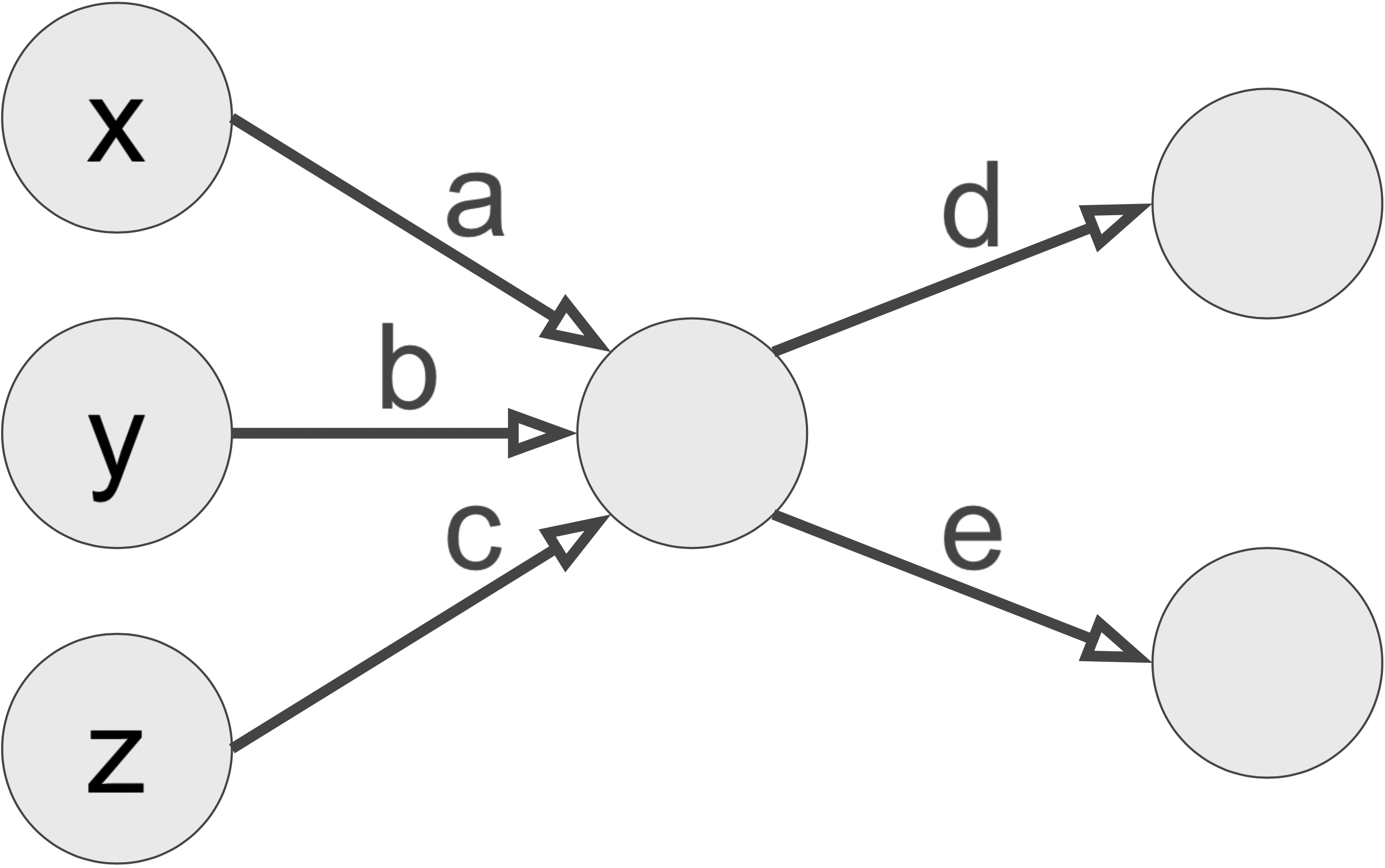
The neuromanifold is a key player in the optimization problem of training a neural network. A fixed neural network architecture parametrizes a set of functions, wherein each choice of parameters gives rise to an individual function. This set of functions is the neuromanifold of the network. For instance, the neuromanifold in Figure 1 is the set of all linear maps \(\mathbb{R}^3 \rightarrow \mathbb{R}^2\) with rank at most one. The neuromanifold in this simple example is a well-studied algebraic variety, but it suggests several tough questions for real-life networks: What is the geometry of the neuromanifold? What does it look like? And how does the geometry affect the training of the network?
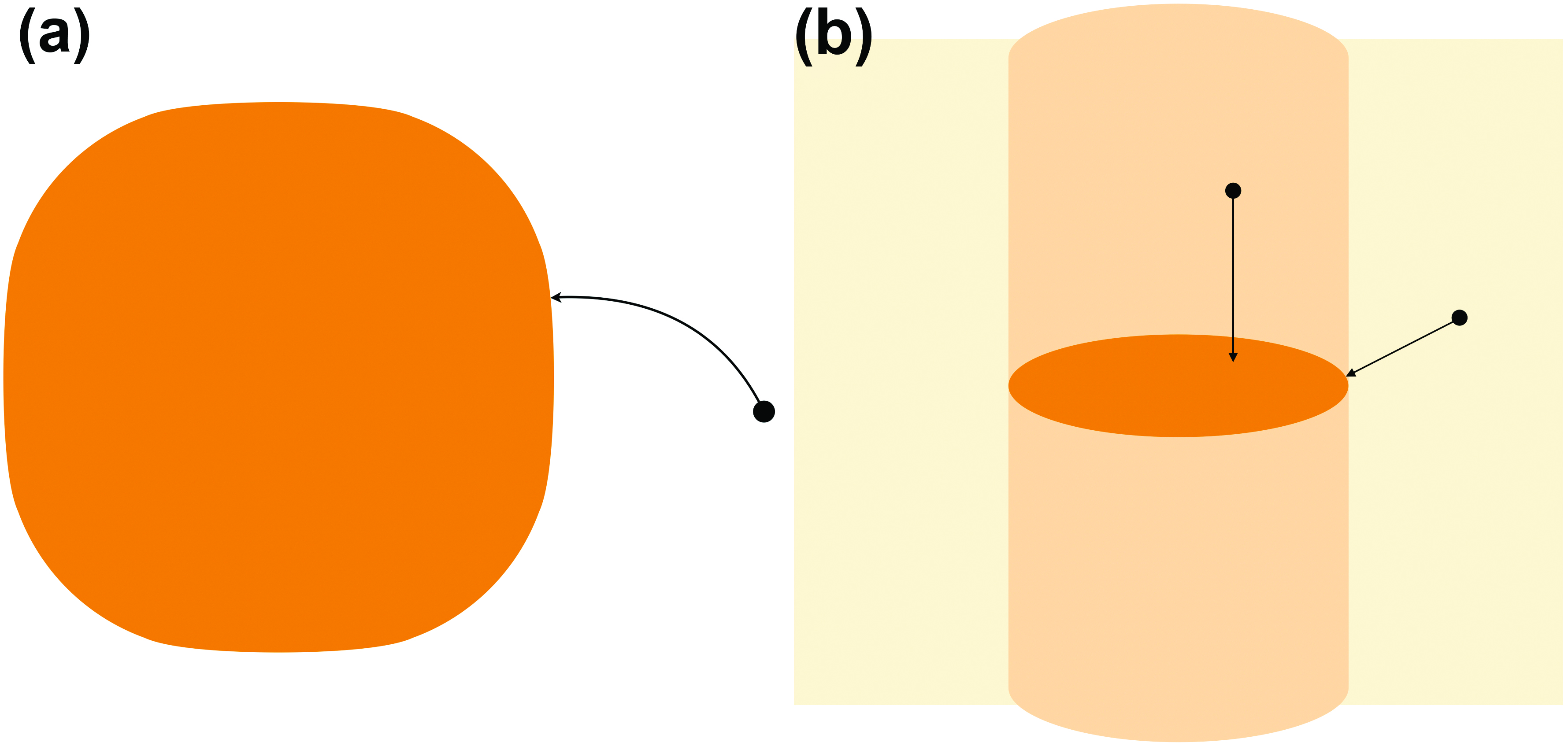
Let us explore another simple example of geometry’s ability to govern optimization. Imagine the neuromanifold as a full-dimensional subset of \(\mathbb{R}^n\) that is closed in the usual Euclidean topology (see Figure 2a). In a supervised learning setting, we provide some training data that is represented as a point in the ambient space \(\mathbb{R}^n\). Independent of the choice of loss function to be minimized, only two scenarios can occur during network training: (i) If the data point is inside the neuromanifold, then that point is the global minimum; or (ii) if the data point is outside of the neuromanifold, then the global minimum lies on the neuromanifold’s boundary. These scenarios have practical consequences. If we can test a point’s membership in the neuromanifold, we can hence reduce the number of optimization parameters by constructing a smaller network that only parametrizes the boundary of the original neuromanifold.
This behavior changes drastically when the neuromanifold is a lower-dimensional subset of its ambient space \(\mathbb{R}^n\). Suppose that the neuromanifold is a closed, two-dimensional disk inside \(\mathbb{R}^3\), and the loss function we want to minimize is the standard Euclidean distance from a given data point. In this case, the global minimum for data points inside the cylinder over the disk will be in the (relative) interior of the neuromanifold, while the minimum for all other points will fall on the (relative) boundary (see Figure 2b). When we alter the loss function, the cylinder changes its shape — which can be challenging to understand.
The boundary points of the neuromanifold are not the only interesting points that can become more exposed during training. A neuromanifold often has singularities: points at which it does not look locally like a regular manifold. For instance, imagine the neuromanifold as the plane curve in Figure 3, which has one singularity: a cusp. Figure 3 illustrates the data points whose global minimum is the cusp during the minimization of the Euclidean distance. This set of data points has a positive measure, which means that the cusp is the global minimum with positive probability over the data. On the contrary, any other fixed nonsingular point on the curve is the minimum with probability zero.
Of course, the neuromanifolds of actual neural networks are more complicated than these toy examples. Their boundary points and singularities are difficult to describe, but—as in the previous examples—they are important for understanding neural network training. In the context of these optimization properties, an additional layer of complexity arises because the network training does not occur in the space of functions where the neuromanifold lives, but rather in the space of the parameters. Different networks can yield the same neuromanifold, but they parametrize that neuromanifold in distinct ways. Such parametrization often induces spurious critical points in parameter space that do not serve as critical points on the neuromanifold in function space [7].
![<strong>Figure 3.</strong> For any point within the pink region, the unique closest point on the purple curve is the red cusp. In the teal region, the red cusp is one of several closest points. Figure courtesy of [1].](/media/y13dt3ic/figure3.jpg)
Among the easiest network architectures to study are fully connected linear networks. This architecture has no activation function, and all neurons from one layer are connected to all neurons in the next layer. As in Figure 1, the neuromanifold of such a network is an algebraic variety (i.e., a solution set of polynomial equations) that consists of low-rank matrices. Though it has no boundary points, it does have singularities (i.e., matrices of even lower rank). Depending on the loss function, these singularities can be critical points with positive probability (see Figure 3). Along with the spurious critical points in parameter space, they play a crucial role in the analysis of the convergence of gradient descent [5].
In a linear convolutional network, not all neurons between neighboring layers are connected, and several edges between neurons share the same parameter. More concretely, this type of network parametrizes linear convolutions that themselves are composed of many individual convolutions: one for each network layer. For instance, a linear convolution on one-dimensional signals is a linear map wherein each coordinate function takes the inner product of a fixed filter vector with part of the input vector (see Figure 4). The composition of such convolutions in a neural network is equivalent to the multiplication of certain sparse polynomials. And unlike the fully connected case, this network’s neuromanifold is typically not an algebraic variety. Instead, it is a semi-algebraic set — i.e., the solution set of polynomial equations and polynomial inequalities (like the disk in Figure 2b) [3]. Moreover, the neuromanifold is closed in the standard Euclidean topology. It typically has a non-empty (relative) boundary whose relevance for network training depends on the network architecture, and particularly on the strides of the individual layers.
The stride of a linear convolution on one-dimensional signals measures the speed at which the filter moves through the input vector. If the linear convolutions in all network layers have stride one, the neuromanifold is a full-dimensional subset of an ambient vector space with no singularities (see Figure 2a). Its boundary points often manifest as critical points, and spurious critical points also frequently appear [3].

If the linear convolutions in all network layers have strides that are strictly larger than one, the dimension of the neuromanifold is smaller than the dimension of the smallest vector space that contains it [4]. The neuromanifold typically has both singularities and boundary points, but—in contrast to all of the other network architectures that we described—they almost never appear as critical points when we train the network via squared error loss (under mild assumptions). More concretely, in the presence of a sufficient amount of generic (i.e., slightly noisy) data, all nonzero critical points of the squared error loss are nonsingular points in the (relative) interior of the neuromanifold [4].
In addition, no nonzero spurious critical points are present in parameter space, which allows us to describe and count all critical points via algebraic methods in function space [6]. Ultimately, the behavior of critical points for linear convolutional networks with all strides larger than one is more favorable than that of linear networks that are fully connected or convolutional with stride one; this is because the latter networks commonly have nontrivial spurious and singular/boundary critical points, at which gradient descent can get stuck.
In conclusion, we can drastically change the geometry of a neuromanifold by varying the architecture of its neural network. For the simple architectures that we describe here, the neuromanifold is a stratified manifold that consists of low-rank matrices/tensors or reducible polynomials. Its geometry governs the optimization behavior during network training. We have demonstrated the impact of replacing fully connected layers with convolutional layers in linear networks; future work will reveal the corresponding effect on nonlinear networks. Interested researchers can use algebro-geometric tools [2] to explore algebraic activation functions, such as the rectified linear unit [8] or polynomial activation. The study of other activation functions will require analytic techniques and collaborations between several mathematical areas.
References
[1] Brandt, M., & Weinstein, M. (2024). Voronoi cells in metric algebraic geometry of plane curves. Math. Scand., 130(1).
[2] Breiding, P., Kohn, K., & Sturmfels, B. (2024). Metric algebraic geometry. In Oberwolfach seminars (Vol. 53). Cham, Switzerland: Birkhäuser.
[3] Kohn, K., Merkh, T., Montúfar, G., & Trager, M. (2022). Geometry of linear convolutional networks. SIAM J. Appl. Algebra Geom., 6(3), 368-406.
[4] Kohn, K., Montúfar, G., Shahverdi, V., & Trager, M. (2024). Function space and critical points of linear convolutional networks. SIAM J. Appl. Algebra Geom., 8(2), 333-362.
[5] Nguegnang, G.M., Rauhut, H., & Terstiege, U. (2021). Convergence of gradient descent for learning linear neural networks. Preprint, arXiv:2108.02040.
[6] Shahverdi, V. (2024). Algebraic complexity and neurovariety of linear convolutional networks. Preprint, arXiv:2401.16613.
[7] Trager, M., Kohn, K., & Bruna, J. (2020). Pure and spurious critical points: A geometric study of linear networks. In 8th international conference on learning representations.
[8] Zhang, L., Naitzat, G., & Lim, L.-H. (2018). Tropical geometry of deep neural networks. In Proceedings of the 35th international conference on machine learning (PMLR) (pp. 5824-5832). Stockholm, Sweden.
About the Author
Kathlén Kohn
Assistant Professor, KTH Royal Institute of Technology, Sweden
Kathlén Kohn is a tenure-track assistant professor at KTH Royal Institute of Technology in Sweden. Her research uses algebraic methods to investigate the underlying geometry in computer vision, machine learning, and statistical problems

Stay Up-to-Date with Email Alerts
Sign up for our monthly newsletter and emails about other topics of your choosing.
