The Mathematics of Reliable Artificial Intelligence

The recent unprecedented success of foundation models like GPT-4 has heightened the general public’s awareness of artificial intelligence (AI) and inspired vivid discussion about its associated possibilities and threats. In March 2023, a group of technology leaders published an open letter that called for a public pause in AI development to allow time for the creation and implementation of shared safety protocols. Policymakers around the world have also responded to rapid advancements in AI technology with various regulatory efforts, including the European Union (EU) AI Act and the Hiroshima AI Process.

One of the current problems—and consequential dangers—of AI technology is its unreliability and subsequent lack of trustworthiness. In recent years, AI-based technologies have often encountered severe issues in terms of safety, security, privacy, and responsibility with respect to fairness and interpretability. Privacy violations, unfair decisions, unexplainable results, and accidents involving self-driving cars are all examples of concerning outcomes.

Overcoming these and other problems while simultaneously fulfilling legal requirements necessitates a deep mathematical understanding. Here, we will explore the mathematics of reliable AI [1] with a particular focus on artificial neural networks: AI’s current workhorse. Artificial neural networks are not a new phenomenon; in 1943, Warren McCulloch and Walter Pitts developed preliminary algorithmic approaches to learning by introducing a mathematical model to mimic the functionality of the human brain, which consists of a network of neurons [10]. Their approach inspired the following definition of an artificial neuron:

\[f(x_1,...,x_n) = \rho\left( \sum_{j=1}^n x_j w_j - b\right), \quad f : \mathbb{R}^n \to \mathbb{R},\]

with weights \(w_1, ..., w_n \in \mathbb{R}\), bias \(b \in \mathbb{R}\), and activation function \(
\rho : \mathbb{R} \to \mathbb{R}\), which is typically the rectified linear unit (ReLU) \(\rho (x)= \max\{0,x\}\). Arranging these artificial neurons into layers yields the definition of an artificial neural network \(\Phi\) of depth \(L\):

\[\Phi(x) := T_L \rho(T_{L-1}\rho(\ldots(\rho(T_1(x)))\ldots)), \quad \Phi : \mathbb{R}^n \to \mathbb{R},\]

where \(T_k (x) = W_k(x) - b_k\), \(k=1, \ldots, L\) are affine-linear functions with \(W_k\) as the weight matrices and \(b_k\) as the bias vectors. It is worth noting that an artificial neural network is indeed a purely mathematical object.

Let us next discuss the workflow for the application of (artificial) neural networks, which automatically leads to key research directions in the realm of reliability. Given a data set \((x_i,y_i)_i\)—which may be sampled from a classification function of data on a manifold \(\mathcal{M}\), i.e., \(g: \mathcal{M} \to \{1,...,K\}\)—the key task of a neural network \(\Phi\) is to approximate the data and the underlying function \(g\). After splitting the data set into a training set and a test set, we can proceed as follows:

(i) Choose an architecture by determining the number of layers in the network, the number of neurons in each layer, and so forth.

(ii) Train the neural network by optimizing the weight matrices and bias vectors. This step is accomplished via stochastic gradient descent, which solves the optimization problem

\[\min_{W_k,b_k} \sum_{i} \mathcal{L}(\Phi_{W_k,b_k}(x_i),y_i) + \lambda \mathcal{R}(W_k,b_k).\]

Here, \(\mathcal{L}\) is a loss function (such as the square loss) and \(\mathcal{R}\) is a regularization term.

(iii) Use the test data to analyze the trained neural network’s ability to generalize to unseen data.

These steps lead to three particular research directions—expressivity, training, and generalization—that are associated with the three error components in a statistical learning problem: approximation error, error from the algorithm, and out-of-sample error.

The area of expressivity seeks to determine approximation properties of the considered class of neural networks with respect to certain “natural” function classes, while also typically accounting for the neural networks’ required complexity in terms of the number of nonzero parameters (weights and biases). Expressivity is perhaps the most thoroughly explored mathematical research direction of AI. An early highlight was the development of the famous universal approximation theorem in the 1980s [6]. This theorem shows that we can approximate any continuous function up to an arbitrary degree for non-polynomial activation functions of shallow neural networks, which were state of the art at the time. Intriguingly, recent results prove that neural networks can simulate most known approximation schemes, including approximation by affine systems like wavelets and shearlets [4].

The difficulty of training stems from the optimization problem’s high nonconvexity and the presence of spurious local minima, saddle points, and local maxima in the loss landscape. It is therefore particularly surprising that stochastic gradient descent seems to find “good” local minima in the resulting generalization performance. Achieving this success requires analysis of the loss landscape via a combination of training dynamics and techniques from areas such as algebraic geometry. One recent highlight is the phenomenon of neural collapse [11], wherein the class features form well-separated clusters in feature space during the final stages of training. This result helped us understand why training beyond the point of zero training error does not yield a highly overfitted model, as we might expect.

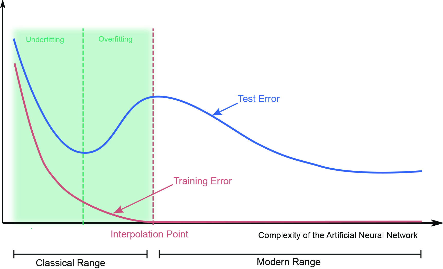
We can essentially subdivide generalization into two classes: functional analytic approaches and stochastic/statistical approaches. The first class typically aims for error bounds in deterministic settings. For example, we can precisely determine the generalization error of spectral graph convolutional neural networks for input graphs that model the same phenomenon, e.g., in the sense of graphons [9]. In contrast, the second class typically seeks to analyze the so-called double descent curve, which exhibits the surprisingly positive effects of overparameterization (see Figure 1). Such analysis usually relies on methods like the Vapnik-Chervonenkis dimension, Rademacher complexity, or neural tangent kernels [7].

A deep mathematical understanding of expressivity, training, and generalization will be crucial to ensure reliability. However, the aforementioned EU AI Act and other similar regulations question whether reliability is achievable without detailed information about the entire training process. These policies ask for a “right to explanation” for AI technologies. Such requests lead to the concept of explainability, which aims to clarify the way in which neural networks reach decisions by determining and highlighting the main features of the input data that contribute to a particular decision. This ability would be highly useful for both explaining decisions to customers and deriving additional insights from data in scientific applications. One goal is to develop explainability approaches that enable human users to communicate with a neural network in the same way that they might communicate with a human; the advent of large language models has brought this vision one step closer to reality. But from a mathematical standpoint, such an approach must also be reliable itself. Several potential mathematically grounded explainability methods are presently available, such as Shapley values from game theory [13] and rate-distortion explanations from information theory [8].

While users are currently applying deep neural networks and AI techniques to a wide variety of problems in science and industry, these methods do have significant limitations. This research direction is unfortunately not a major focus at the moment, but some results are still worth highlighting. For example, recent work demonstrated that the minimal number of training samples to guarantee a given uniform accuracy on any learning problem scales exponentially in both the depth and input dimension of the network architecture; this means that learning ReLU networks to high uniform accuracy is intractable [2]. In 2022, another study analyzed the problem of running AI-based algorithms on digital hardware (like graphical processing units) that is modeled as a Turing machine, whereas the problems themselves are typically of a continuum nature [5]. Unfortunately, this discrepancy makes various problems—including inverse problems—noncomputable and causes serious reliability issues. At the same time, other results indicate that Blum-Shub-Smale machines—which relate to innovative analog hardware, such as neuromorphic chips or quantum computing—could surmount this obstacle [3]. Such hardware will hopefully also overcome the acute concern of energy consumption by digital hardware (see Figure 2), which is a key item in the U.S. CHIPS and Science Act.

To summarize, unreliability is one of the most serious impediments in the development of AI technology, and many areas of mathematics will help address this complication. Furthermore, the automatic verification of properties that are legally required for AI-based approaches is only attainable through a mathematization of terms like the “right to explanation.” AI reliability is hence inextricably linked to mathematics, ultimately creating very exciting research opportunities for our community.

References

[1] Berner, J., Grohs, P., Kutyniok, G., & Petersen, P. (2022). The modern mathematics of deep learning. In P. Grohs & G. Kutyniok (Eds.), Mathematical aspects of deep learning (pp. 1-111). Cambridge, U.K.: Cambridge University Press.
[2] Berner, J., Grohs, P., & Voigtlaender, F. (2023). Learning ReLU networks to high uniform accuracy is intractable. In The eleventh international conference on learning representations (ICLR 2023). Kigali, Rwanda.
[3] Boche, H., Fono, A., & Kutyniok, G. (2022). Inverse problems are solvable on real number signal processing hardware. Preprint, arXiv:2204.02066.
[4] Bölcskei, H., Grohs, P., Kutyniok, G., & Petersen, P. (2019). Optimal approximation with sparsely connected deep neural networks. SIAM J. Math. Data Sci., 1(1), 8-45.
[5] Colbrook, M.J., Antun, V., & Hansen, A.C. (2022). The difficulty of computing stable and accurate neural networks: On the barriers of deep learning and Smale’s 18th problem. Proc. Natl. Acad. Sci., 119(12), e2107151119.
[6] Cybenko, G. (1989). Approximation by superpositions of a sigmoidal function. Math. Control Signals Syst., 2, 303-314.
[7] Jacot, A., Gabriel, F., & Hongler, C. (2018). Neural tangent kernel: Convergence and generalization in neural networks. In NIPS’18: Proceedings of the 32nd international conference on neural information processing systems (pp. 8580-8589). Montreal, Canada: Curran Associates, Inc.
[8] Kolek, S., Nguyen, D.A., Levie, R., Bruna, J., & Kutyniok, G. (2022). A rate-distortion framework for explaining black-box model decisions. In A. Holzinger, R. Goebel, R. Fong, T. Moon, K.-R. Müller, & W. Samek (Eds.), xxAI - Beyond explainable AI (pp. 91-115). Lecture notes in computer science (Vol. 13200). Cham, Switzerland: Springer.
[9] Levie, R., Huang, W., Bucci, L., Bronstein, M., & Kutyniok, G. (2021). Transferability of spectral graph convolutional neural networks. J. Mach. Learn. Res., 22(1), 12462-12520.
[10] McCulloch, W.S., & Pitts, W. (1943). A logical calculus of the ideas immanent in nervous activity. Bull. Math. Biophys., 5, 115-133.
[11] Papyan, V., Han, X.Y., & Donoho, D.L. (2020). Prevalence of neural collapse during the terminal phase of deep learning training. Proc. Natl. Acad. Sci., 117(40), 24652-24663.
[12] Semiconductor Research Corporation (2021). Decadal plan for semiconductors: Full report. Durham, NC: Semiconductor Research Corporation. Retrieved from https://www.src.org/about/decadal-plan.
[13] Štrumbelj, E., & Kononenko, I. (2010). An efficient explanation of individual classifications using game theory. J. Mach. Learn. Res., 11(1), 1-18.